
Building the SUAS Search Simulator
Why we started with a simulator
Before ASCENT-1 ever flies a search pattern at SUAS 2026, we wanted a way to answer one question honestly: which search strategy finds the targets fastest without draining the battery? This is our first real piece of AI engineering for the competition, a simulator that lets us try search algorithms against the actual SUAS 2026 mission area and see how they do, long before any of them touch the aircraft.
Pick the wrong search pattern and you pay for it three times over wasted battery, a longer mission, and a smaller chance of actually spotting the targets. We did not want to choose on a hunch, and flight testing on its own cannot settle it: real flights are expensive, they depend on the weather, they are hard to repeat exactly, and there is no way to fly the hundreds or thousands of scenarios you would need to trust the answer. The occlusion problem makes it harder still, because flying over a target is not the same as seeing it and any fair test has to tell those two things apart.
How the simulator is put together
We built the simulator as a handful of small pieces, each doing one job, with information flowing in one direction — from the real mission map at the top down to the metrics at the end. Here is what each piece does.
It starts with the real map
Everything begins with the official Google Earth KML that RoboNation publishes for the competition — not a map we drew ourselves. That gives us the genuine flight boundary, both search boundaries, the runways, and the team operation areas, laid out in a local ENU coordinate system.
The aircraft
The drone model stands in for ASCENT-1: how fast it flies and the limits on how it can move. It gives the simulation something realistic to fly, so a path that looks good on paper still has to obey the same constraints the real aircraft would.
The camera
The camera model describes what the aircraft can actually see — its field of view and the patch of ground it covers at a given altitude. That footprint is the starting point for two things: how much ground we have imaged, and whether a target sitting inside that patch actually gets detected.
Covering ground isn't the same as seeing a target
This is the part we care about most. It is tempting to assume that if you fly over something you have found it — but the handbook says the mannequin can be tucked under bushes or behind a vehicle, so that assumption falls apart fast. So we split the problem in two: one part tracks the geometry of which ground we imaged (that is the coverage number), and a separate part decides whether a target in that area was really spotted, taking occlusion, image resolution, and range into account. Keeping them apart means an algorithm is judged on what it would actually detect, not just how much dirt it flew over.
Search algorithms you can swap out
Every search algorithm plugs into the same slot. Because they all share one interface, the rest of the simulator does not know or care which one is running — so we can add a new strategy and test it without touching anything else.
Keeping the pieces independent
The whole thing is layered so that dependencies only ever point one way — from the configuration at the top, down through the experiments, metrics, simulator, algorithms, and the world, drone, and camera models, to a small set of shared utilities at the bottom. In short, the flow looks like this:
Official KML → Map Parser → World Model → Drone Model → Camera Model →
Coverage Engine → Simulation Engine → Search Algorithm → Evaluation Framework
One deliberate choice: the competition flight software is kept out of this core completely. The eventual stack — ArduPilot, MAVLink, Jetson Nano, and YOLO — has no place in the simulator itself. When the time comes it will connect through adapters on the edges, so none of it can tangle up the part that does the evaluation.
The reason we made everything plug-compatible is exactly this: we can keep adding search strategies and put them through the same tests without rewriting the map handling, the simulation, or the scoring. That is what makes this a testbed we can grow, instead of a one-off built around a single idea.
How we score a run
Instead of eyeballing which run looked better, every mission is scored on hard numbers. Right now we track:
- Mission completion time
- Time to first target detection
- Total flight distance
- Estimated battery consumption
- Coverage percentage
- Coverage efficiency
- Redundant coverage
- Number of turns
- Mission success rate
- Search efficiency
The point of all this is comparison at scale. We run each algorithm across large Monte Carlo campaigns — the targets get dropped in random spots and the mission is flown over and over. Anything random in the simulation runs off a seed we save with the result, so if a run does something surprising, we can replay it exactly and figure out why.
What the early runs are telling us
The whole reason the simulator exists is to swap opinions for measurements, so once it worked we put it straight to work. We have run early campaigns of 1,000 missions per algorithm over the real mission area at 45.72 m (150 ft) AGL, plus a sensitivity study that nudges one mission setting at a time to see what actually moves the numbers. Each campaign gives us a composite score, the per-metric figures behind it, and a sense of how steady each algorithm's ranking is.
Here is a representative snapshot from one 1,000-mission campaign. One word of caution before reading too much into it: these numbers are here to show the framework can tell planners apart on time, distance, energy, and efficiency — they are not us crowning a winner, and several of the algorithms in the list are still being built.
| Rank | Algorithm | Score | Success % | Coverage % | Time (s) | Energy (Wh) | Search eff. (m²/s) |
|---|---|---|---|---|---|---|---|
| 1 | Lawnmower | 0.964 | 100.0 | 100.0 | 56.5 | 5.5 | 689.3 |
| 2 | Hybrid | 0.705 | 97.6 | 98.7 | 51.0 | 5.0 | 751.2 |
| 3 | InfoGain | 0.592 | 98.0 | 98.8 | 64.5 | 6.3 | 600.8 |
| 4 | AdaptiveGrid | 0.475 | 96.5 | 98.5 | 76.0 | 7.4 | 505.7 |
| 5 | Spiral | 0.461 | 97.7 | 98.5 | 72.0 | 7.0 | 531.5 |
| 6 | NBV | 0.380 | 97.1 | 98.6 | 110.6 | 10.7 | 349.3 |
| 7 | Bayesian | 0.380 | 97.1 | 98.6 | 110.6 | 10.7 | 349.3 |
| 8 | Random | 0.108 | 100.0 | 98.8 | 258.3 | 25.1 | 171.2 |
Preliminary output from a Monte Carlo campaign (1,000 missions per algorithm, cell size 10 m, 45.72 m AGL, 18 m/s, 120 Wh battery, 70° HFOV). Used to validate the evaluation framework; it does not represent a final algorithm choice.
We also look at how each algorithm holds up across every configuration we tried, not just one — its average ranking and how much that ranking bounces around:
| Algorithm | Mean rank | Rank std | Best | Worst |
|---|---|---|---|---|
| Lawnmower | 1.33 | 0.94 | 1 | 5 |
| Hybrid | 1.89 | 0.46 | 1 | 3 |
| InfoGain | 3.44 | 0.83 | 2 | 5 |
| AdaptiveGrid | 4.22 | 1.03 | 3 | 7 |
| NBV | 5.33 | 1.15 | 2 | 6 |
| Spiral | 5.44 | 1.12 | 3 | 7 |
| Bayesian | 6.33 | 1.15 | 3 | 7 |
| Random | 8.00 | 0.00 | 8 | 8 |
Lower mean rank is better on average; lower rank standard deviation indicates greater robustness to configuration.
So far the steady, cover-everything patterns are doing well — both on efficiency and on staying consistent — while several of the smarter probabilistic planners still need to be written and tuned before it is a fair fight. We have not picked a final algorithm for ASCENT-1 yet, and we are not going to until the evidence says so. That is the whole reason we built this.
Figures
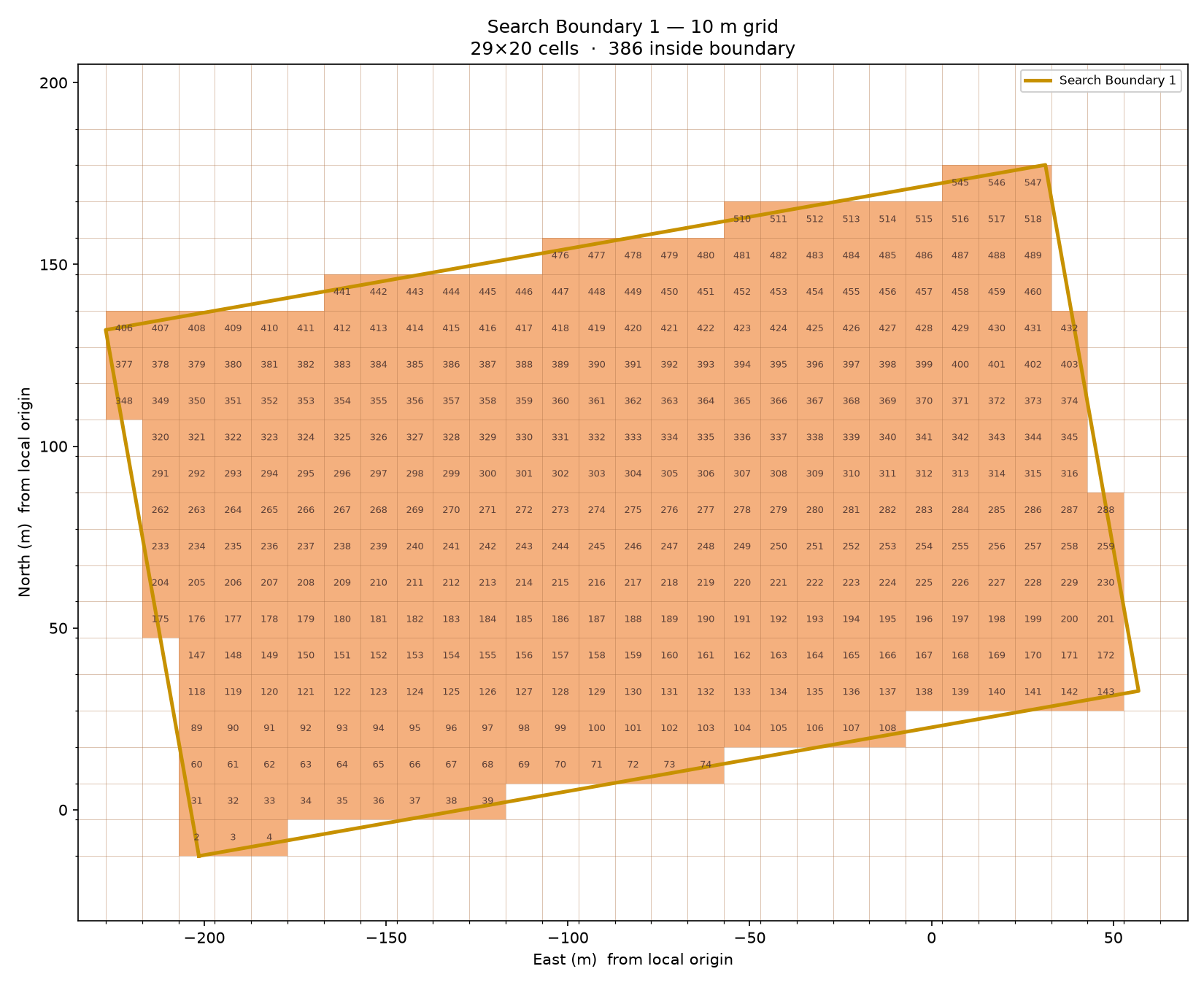
Search Area Grid
Official SUAS 2026 mission environment imported directly from the RoboNation KML.
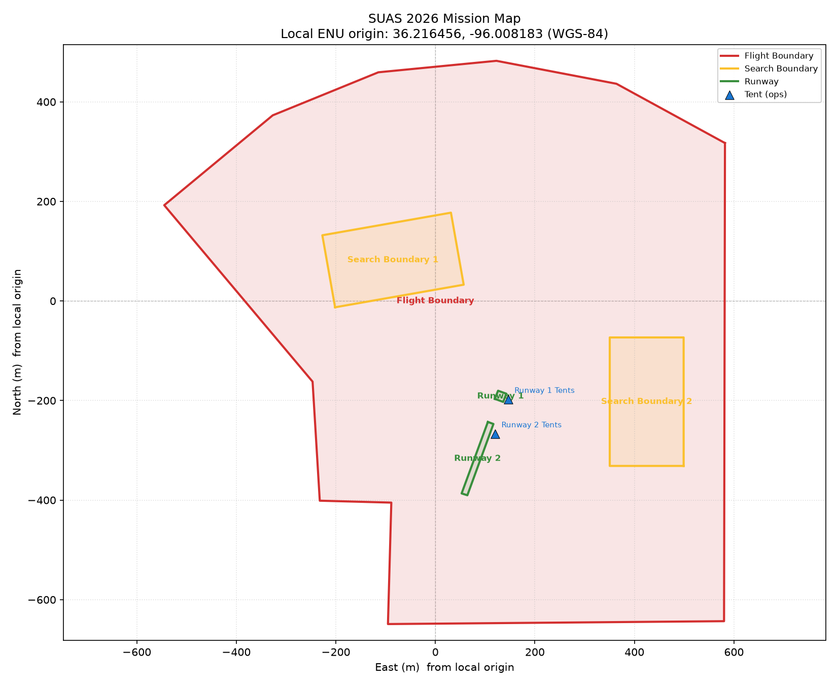
Mission Map Preview
Visualization of the official search boundaries, flight boundaries, and operational areas used by the simulator.
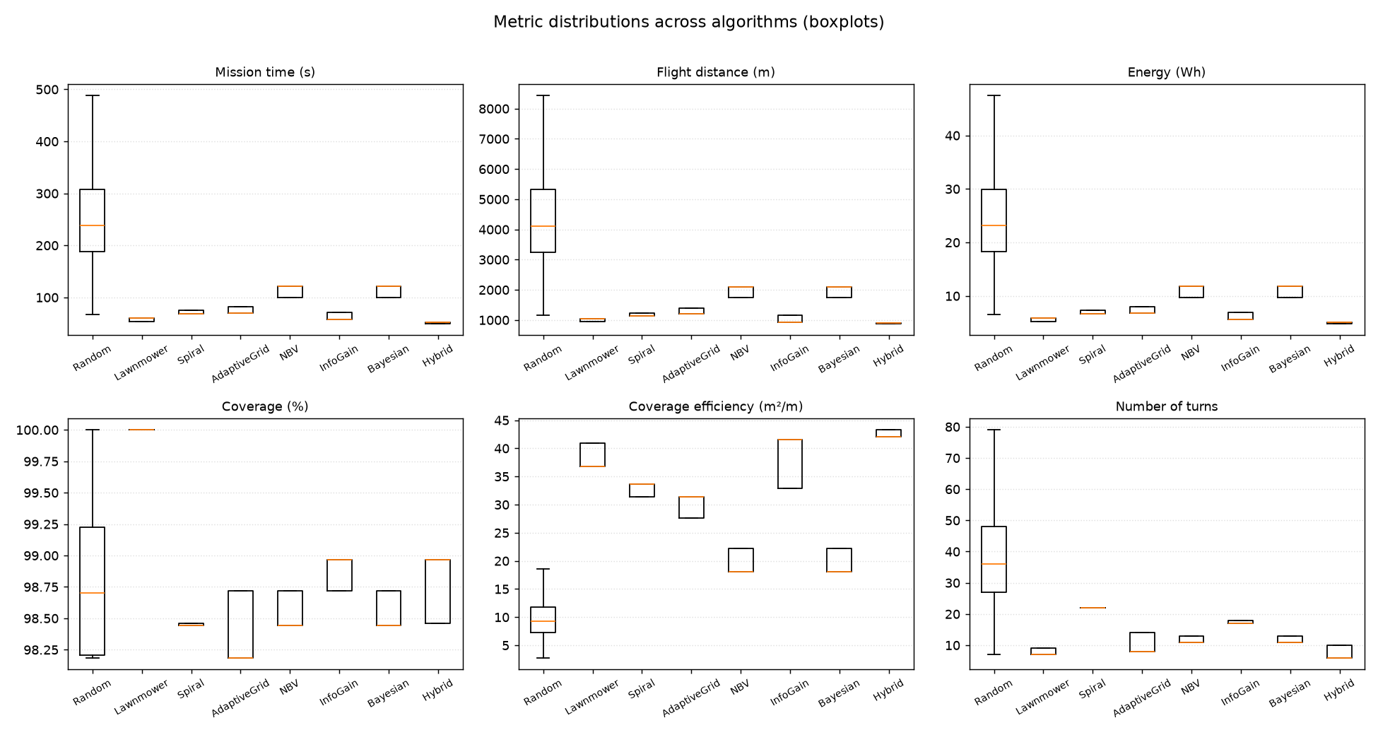
Algorithm Comparison
Statistical comparison of implemented search algorithms using mission completion metrics tailored to the ASCENT-1 platform.
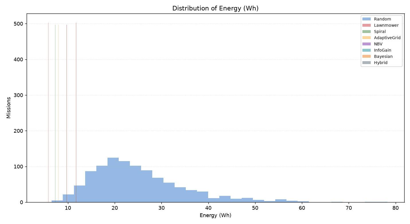
Battery Consumption Histogram
Estimated battery utilization across simulation runs for evaluating mission endurance and energy efficiency.
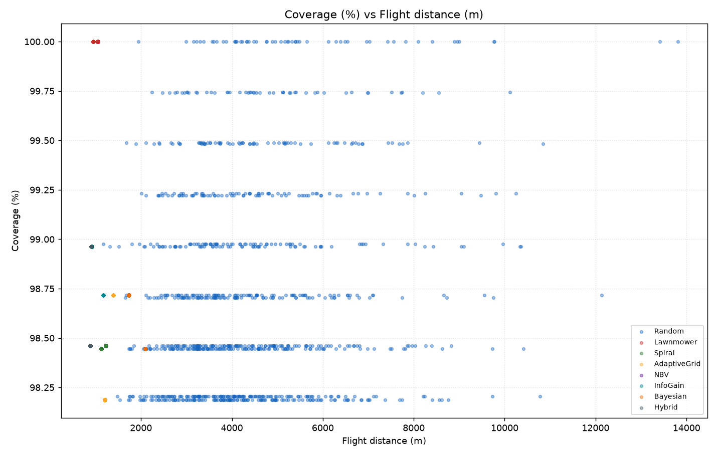
Coverage vs Distance
Relationship between search coverage and total flight distance for different autonomous search strategies.